Refuting the ice volume proxy by system dynamics.

Abstract
Oxygen isotope (δ18O) data collected from ocean sediment cores (benthic stacks) are thought to be a proxy for global ice volume during the Pleistocene ice ages. However, the ‘system dynamics’ of accumulating ice sheets causes a phase shift compared to the original forcing signal, which is thought to be represented by the Antarctic temperature reconstruction from the ice cores. when this heavier seawater (containing more of the heavy O and H isotopes) sinks to the ocean floor, secondary dynamic modification of the signal should take place (mixing, diluting) . However, these processes cannot be inferred from the actual isotope signals of the benthic foraminifera records. Instead they closely resemble the original assumed input signal (r2=81%). The conclusion is that the isotopes in the benthic stacks did not follow the dynamics of ice sheet accumulation and distribution processes within the ocean, hence they cannot be representing global ice sheet volumes.
Samenvatting
Isotoopverhoudingen (δ18O) in sedimentkernen van de oceaanbodem (benthic stacks) worden verondersteld een proxy te zijn voor globaal ijsvolume tijdens de Pleistocene ijstijden. De dynamica van groeiende ijskappen veroorzaakt echter een faseverschuiving in het output signaal ten opzichte van de oorspronkelijke forcing-functie, de reconstructie van de Antarctische temperatuur uit de ijskernen. Een tweede dynamische modificatie van het signaal zou moeten plaatsvinden wanneer het zwaardere zeewater, de bron van de verdamping, naar de oceaanbodem gaat. Deze processen kunnen echter niet worden afgeleid uit de werkelijke isotopensignalen van de benthische foraminifera stacks. In plaats daarvan lijken ze sterk op de oorspronkelijke input, (r2 = 81%). De conclusie is dat de isotopen in de bentische stacks noch de dynamiek van de accumulatie van het poolijs, noch de dynamiek van de verspreidingsprocessen van isotopen in de oceaan kunnen hebben gevolgd, en daarom kunnen ze geen proxies zijn voor globale ijsvolumes.
Introduction
In our previous contribution we have seen that several proxies for the ice ages failed to indicate an exceptional warm period some 50,000 years ago, closely resembling an interglacial (fig 1). Neither the temperature (blue) or CO2 (green) reconstructions from the ice cores in Antarctica, nor the temperature/ice volume reconstruction from the foraminifera isotopes, the benthic stack LR04[i] (black) demonstrated any such occurrence.
The revised integrated summer insolation for the Northern hemisphere did show this interglacial-like interval (MIS-3), suggesting that this is a much better indicator for climate from the past. However the lockstep of the two previously mentioned isotope records of inferred temperature from Antarctic ice cores and ocean foraminifera records (blue and black) is striking, despite their totally different properties. Yet they both failed to record the high temperatures of MIS-3. Consequently, these isotope-records may be signalling something else. We will investigate that in a forthcoming article. For now,we will demonstrate that the dynamic system logic of this ice age hypothesis is in error.
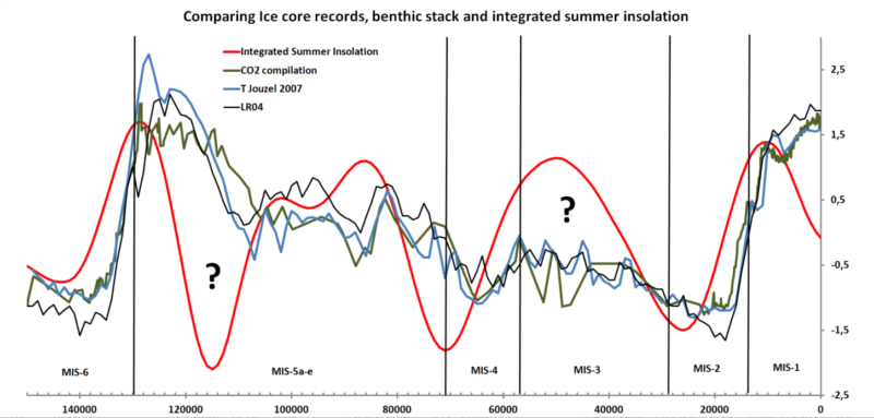
Fig 1 Comparing CO2, isotopes and insolation
Starting in the 1950s, an extensive ocean drilling program (ODP) was carried out, collecting numerous sediment cores around the world. These core contained fossil shells of foraminifera, constructed by organisms precipitating calcium ions and carbonate ions originating from carbon dioxide, to form calcium carbonate. The oxygen isotope ratio of the carbonates are in dynamic equilibrium with the seawater and hence it was considered to represent the oxygen isotope ratios of the past, modified by local temperature and isotope ratios from the source, the seawater. The δ18O variation was considerable. However, temperature variation in the deep sea is very small, so most of the variation was attributed to concentration differences in the seawater. This in turn was thought to be caused by glaciation (Shackleton 1967).
As heavy isotopes in H2O (18O, 2H) resist evaporating a bit more than the light isotopes (16O, 1H), the ratio of δ18O in the water vapor is slightly lower, leaving heavier isotopes behind in the surface water. This lighter water evaporating from the oceans snowed down and accumulated as more ice on the ice sheets during glacial periods. At the same time, the ocean water remaining in the ocean basin would gradually become enriched in the heavier O and H isotopes, and that process is thought to be visible in the oceanic sediment cores and compilations thereof (Benthic stacks) like SPECMAP of Imbrie et al 1984 . LR04 is the currently prevailing Benthic stack. This process would explain the considerable correlation between isotopes from Antarctic ice cores, thought to represent temperatures, and the isotopes in foraminifera from ocean mud, thought to represent ice volumes, which is elaborately explained in ‘Ice Ages, solving the mystery‘ by Imbrie & Imbrie. However there is a slight problem with this view.
Dynamics of accumulation processes
When ice sheets are growing or receding due to low or high temperatures this is an ongoing accumulating process, not a straight forward linear or proportional process. The rate of growth is depending on temperature (and humidity), hence one could describe the volume of the ice sheet at time t in the most simple way with Ice.Volume(t)=Ice.Volume(t-1) + growing.constant * (t-t0), where t0 represents the balancing temperature at which neither snow/ice accumulation nor melting takes place. The very basics of this function are demonstrated in fig 2.
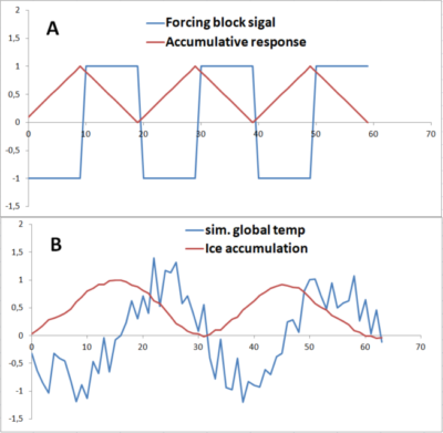
Fig 2 Demonstrating accumulative responses on A: block function, B: harmonic function with simulated noise ripple
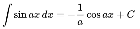
In fig 2A, we start off at t=0 with temperature (blue) at -1 and we see the response of this ‘system’ (red) accumulate linearly until the forcing (‘block’) function swaps at t=10 from minimum to maximum and as a consequence the response function decreases until the next swap at t=20, etc, etc. Obviously as long the temperature is below the balance point, the ice sheets remain accumulating to the highest point at the swap from minimum to maximum. In fig 2B we use the same system function, however now the forcing temperature signal (blue) is a harmonic (sine) with a random noise ripple superimposed, to suggest a more natural process. We note a similar response function (red), simulating ice accumulation. Note again that the ice volume reaches a maximum at the moment that the temperature switches from negative to positive around 16 time units and consequently it reaches a minimum when the temperature drops below zero again. This is not a time delay; it’s just the phase shift of an accumulating or integrating process to the original forcing function. And also obvious from basic mathematics as accumulation functions are represented as integral, and the integral of the sine is a cosine, which is a sine phase shifted with 0.5π (90°):
A second feature to note is the noise on the forcing temperature function, which is highly suppressed on the ice accumulation output.
Of course this is a strong simplification of reality which may include many non linear and stochastic processes and this model does not pretend to simulate reality. It merely demonstrates the dynamics of accumulating processes, especially the phase shift.
Emulation of basic ice sheet accumulation processes
If we apply the same accumulation logic to the temperature reconstruction of Antarctica (blue) [Jouzel [ii]], assuming ice accumulation rate (red) proportional to the temperature reconstruction, using zero as balancing temperature we would get the result in fig.3
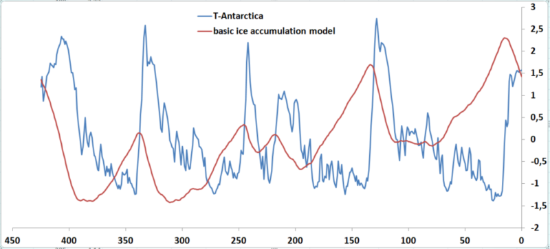
Fig 3 comparing Antarctica ice core temp reconstruction as forcing function for modeled ice accumulation as output (see caption fig 2). Time axis in 1000 of years.
We notice the phase shift again as in fig 2 between the blue forcing and the red response and the ice sheet accumulated minimums are lagging often several thousands of years on the temperature high spikes during the assumed interglacials. Moreover short term cycles are subdued in the output signal as seen in fig 2B. Note that this is just emulating global ice volume, assuming a linear relationship with global temperature.
Simulation of basic oceanic accumulation
The next thing is the question of how the ice volume signal could end up in the foraminifera of the benthic stacks. Obviously this starts with the ocean surfaces, where the evaporation of the lighter isotopes takes place, leaving behind the heavier isotopes δ18O which would accumulate in lockstep with the ice volume. Somehow this heavier water has to sink to the ocean floor and gradually spread throughout all oceans and mix with original water in a second cumulative process with significantly more delay before the foraminifera could capture the heavier isotopes. Hence that red ice volume output signal in fig 3 would undergo a second accumulation process, which would result in something like the green signal in fig 4, depending on choice of parameters. However this appears not to be happening. The δ18O isotope signal in the benthic foraminifera stack LR04 in fig 3 in red is clearly leading the ice volume signal, not to mention any modification of a second accumulation process in the ocean.
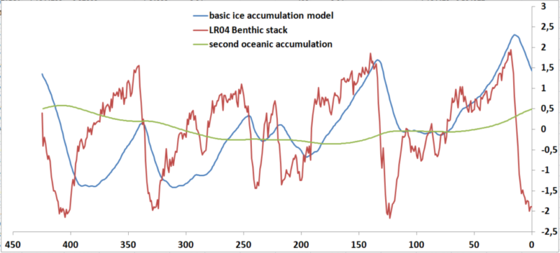
Fig 4 comparing basic simplified ice sheet volume modelling (blue) with further basic simplified dispersion in the oceans (green) with the benthic stack LR04.
If we invert the Bentic stack data and compare it to the temperature reconstruction of Antarctica (fig 5), we observe a striking similarity (r2=81%), even the higher frequency variation, which tends to be subdued in accumulative processes(fig 1b), correlates substantially. Hence the inverted LR04 stack does not show any modification that would have occurred during ice volume accumulation and distribution of δ18O enriched ocean surface waters over the ocean floors and consequently, it can’t represent ice volumes.
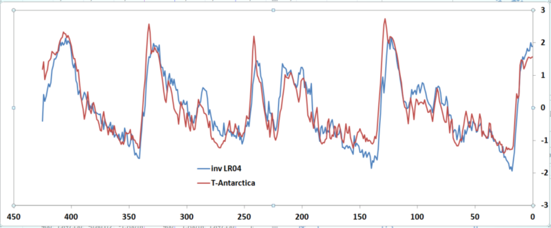
Fig 5. LR04 benthic stack (inverted) versus Antarctic ice core temperature reconstruction on normalized scales on 1000 years time interval.
Conclusion
From this we conclude that the benthic stack LR04 is too directly tied to the alleged Antarctic temperature reconstruction and it does not even remotely resemble logical natural responses from the processes of gradual ice sheet accumulation and distribution of heavy isotope enriched surface water over the deep ocean floor. Instead, its very high correlation with the alleged temperature reconstruction of Antarctica (r2=81%) suggests a direct proportional relationship. Hence the mechanism for both records must be totally different and this implies that isotopes in benthic foraminifera are not related to global ice volume.
In the next article, we will look at the cause(s) of the strong correlation between benthic stacks and Antarctic isotopes.
Notes and references
[i]Lisiecki, L. E., and M. E. Raymo (2005), A Pliocene-Pleistocene stack of 57 globally distributed benthic δ18O records, Paleoceanography, 20, PA1003, doi:10.1029/2004PA001071
[ii] Jouzel, J., et al (32 authors) 2007. Orbital and Millennial Antarctic Climate Variability over the Past 800,000 Years. Science, Vol. 317, No. 5839, pp.793-797, 10 August 2007.
Calculations and graphs (excel2007): online-unsolving
second version (added variable ice sheet growth):online-unsolving-var-growth
Still the “This image was hotlinked”-problem, unlike with any other global blog I follow.
Now it’s good!
I’ve been asked what the significance all this has for climate change.
Check out “The Discovery of Global Warming; Past Climate Cycles: Ice Age Speculations”. https://history.aip.org/climate/cycles.htm
The abstract:
We demonstrated that those cycles did not follow the proposed logic and hence can’t represent glacial cycles. It’s much more ‘dauntingly complex‘
Dear Andre Bijkerk, You did a very good job and your article above makes this clear on a physical basis. Now I am eager to read about implications of this finding. Frans van den Beemt
Thanks, Frans. My idea is that whatever happened, happened at the deep ocean floor first, thinking of tectonics and oceanic volcanism, maybe controlled by forces, (partly) generated by the Milankovitch cycles, but there is still that unsolved 100,000ka Unmilankovitch cycle.
I’ll try to address all that in the next week.
Dear Andre,
I follow your contributions on this subject with great interest, and think it is highly relevant for the ongoing debate.
Reading the above contribution though, a question came up. The ice accumulation model makes use of a growing constant, or growth rate. You note this value depends on temperature and humidity. Could you explain what drives the use of a certain value for growth rate in the model used for the reconstructions above? Could it be that a much higher value, i.e. much more rapid ice accumulation, results in a signal that follows the temperature reconstruction much more closely?
Thanks in advance and kind regards,
Rob
Thanks for the question. Rob. To answer that yourself, you might want to download that excel sheet that’s linked under “online-unsolving”.
Now under the tab “Accumulation proces demo”, we look at the f-column where the ice accumulation response is generated for the sine+ripple function in the graph of fig 2b. You’ll see in field F6 = F5-F$4*E7 Obviously F5 is the previous value, consistent with accumulation. E7 is the forcing function and F$4 is the ‘growing constant’, currently set at 0.1. Now change F4 to anything else, for instance 0.2 and you will see that that the amplitude has doubled, but the phase shift did not change. So the reasoning remains valid at any value of the growing constant.
This also follows from the integral function where the constant a in sin(ax) goes to 1/a after applying the integral.
Dear Andre,
Thanks for your swift response. I tried your suggestion modifying the spreadsheet values, and it does confirm your described behavior (what else did I expect!).
My question is also about the notion that the ice volume keeps accumulating as long as temperatures are low enough. I would assume that an expanding ice sheet will stop expanding at some point, simply due to the fact that it reaches lower latitudes, at which the temperature is still too warm for an ice sheet to be sustained, thereby capping the accumulated ice volume. Of course, this cap would have a specific value for each global temperature, as lower global temperatures allow expansion of the ice sheet further south than warmer temperatures.
If we let your model growing constant be very high, so that it responds to lowering temperatures very quickly by accumulation, but at the same time, cap the accumulated volume due to the maximum ice sheet expansion for each global temperature, wouldn’t you then arrive at a curve that follows the temperature much more closely?
Thanks again,
Rob
Rob,
I’m trying to give a more satisfactory answer. I uploaded a new spreadsheet where de growth constant was made variable as function of the total ice volume. Assuming that initial build up is slower, then acceleration -as the orographic effect on the ice sheet kicks in- and the temperatures drop even more due to its height, and then the final build up slows down again as ablation rate approaches accumulation. I used a simple inverted square function with a maximum at 0.5 (graph below graph B). Note that the result is not that different. The phase shift is still the same.
Rob,
As I suggested indeed reality is much more complicated than we may imagine. For some of these complications I would suggest Mix & Ruddiman 1984; Oxygen-Isotope Analyses and Pleistocene Ice Volumes, QR 21, 1-20 (pay walled) who deal with a lot more of those complexities. For instance the d18O isotope ratio change during ice sheet build up, which would have effect in the other direction i.e. a more gradual change in oceanic d18O. I refrained referring to that, avoiding to scare off the average reader. But even they predict a bigger lag than the much younger LR04 Benthic stack shows.